Gabor–Granger Pricing Model

1. What Is the Gabor–Granger Pricing Model?

The Gabor–Granger Pricing Model is a research technique used to estimate demand at different price points by asking prospective customers about their purchase intent as price changes. By systematically collecting “would you buy?” responses across a predefined set of prices, teams derive an empirical demand curve and identify revenue- or margin-maximizing prices.

In pricing, channel, and sales contexts, it is a practical tool to set list prices, promotional floors, and MSRP guidance for relatively simple offers. It is especially useful when you need quick, directional readouts to inform decisions but lack robust in-market data.

Consultants and executives value Gabor–Granger because it’s fast, intuitive, and actionable. While it does not model multi-attribute trade-offs (like conjoint/discrete choice), it delivers a clear view of how purchase likelihood changes with price—enough to establish an initial price corridor and a working recommendation to validate in market.

2. Origin and Background

Origin: The approach was developed by economists André Gabor and Clive Granger; in use since at least the 1960s.

Why it was created: Marketers and economists needed a simple way to quantify price sensitivity without running full market experiments. Gabor–Granger turned a core behavioral question—“Would you buy at this price?”—into a structured method that produces a demand curve from survey responses.

How it became widely known: It spread through academic literature and research practice, and was adopted by market research firms as a standard pricing module. Over time, it became a staple alongside other tools such as Van Westendorp’s Price Sensitivity Meter and conjoint analysis, each serving distinct use cases.

3. How the Gabor–Granger Pricing Model Works

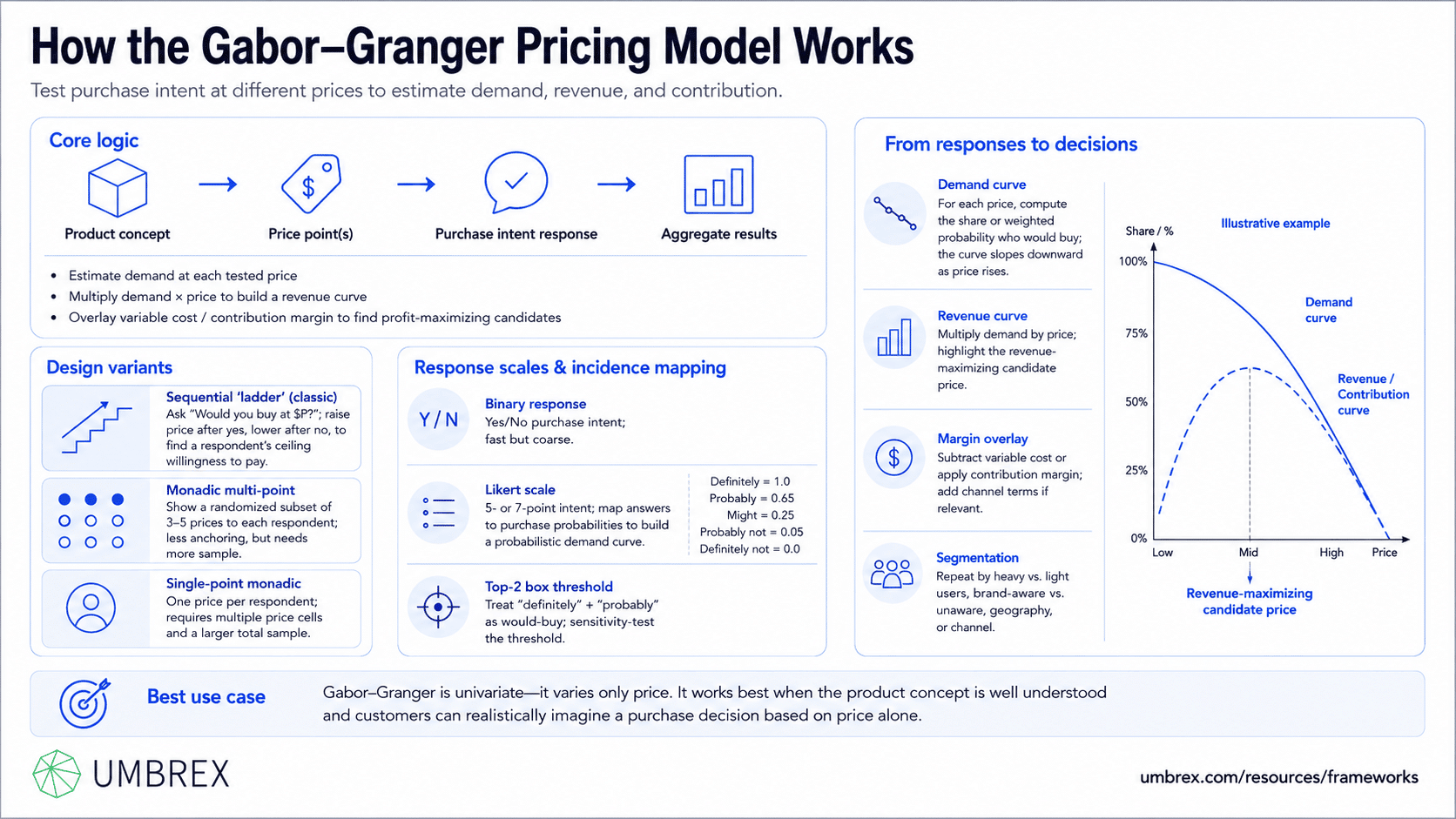
At its core, Gabor–Granger is simple: show a clear product concept, present one or more price points to a respondent, and record their purchase intent at those prices. Aggregate across respondents to estimate the share who would buy at each price. This gives you a demand curve; multiplying by price yields a revenue curve. With margin overlays, you can find the price that maximizes contribution.

Design Variants

• Sequential “ladder” (classic): Ask “Would you buy at $P?” If “yes,” raise the price and ask again until “no.” If “no,” lower the price until “yes” or you hit the floor. This efficiently finds an individual’s “ceiling” willingness to pay.
• Monadic multi-point: Show each respondent a randomized subset of prices (e.g., three to five) and capture intent at each. This reduces anchoring but requires more responses.
• Single-point monadic: Show one price to each respondent and ask purchase intent. You need a larger sample with multiple price cells to build the curve.

Response Scales and Incidence Mapping

• Binary response: Yes/No to “Would you buy?” Fast to field, but coarse.
• Likert scale: 5- or 7-point intent (e.g., “definitely,” “probably,” “might,” “probably not,” “definitely not”). Map the scale to purchase probabilities (e.g., 1.0 for “definitely,” 0.6–0.7 for “probably,” 0 for “not”) to construct a probabilistic demand curve.
• Top-2 box threshold: Treat “definitely” and “probably” as “would buy” to approximate demand; sensitivity-test thresholds.

From Responses to Decisions

• Demand curve: For each price, compute the share (or weighted probability) who would buy. The curve should slope downward as price rises.
• Revenue curve: Multiply demand at each price by the price. The peak is your revenue-maximizing price candidate.
• Margin overlay: Subtract variable cost or apply contribution margin to find profit-maximizing price candidates. Overlay channel terms via a price waterfall if relevant.
• Segmentation: Repeat the analysis by segment (e.g., heavy vs. light users, brand-aware vs. unaware, geography, channel) to tailor pricing or packaging.

Gabor–Granger is univariate—it varies only price. It is strongest when the product concept is well understood and customers can reasonably imagine a purchase decision based on price alone.

4. When to Use the Gabor–Granger Pricing Model

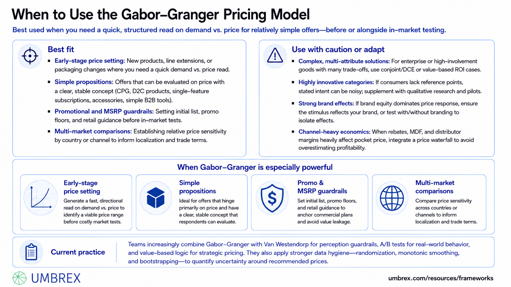
Especially powerful when:

• Early-stage price setting: New products, line extensions, or packaging changes where you need a quick demand vs. price read.
• Simple propositions: Offers that can be evaluated on price with a clear, stable concept (CPG, D2C products, single-feature subscriptions, accessories, simple B2B tools).
• Promotional and MSRP guardrails: Setting initial list, promo floors, and retail guidance before in-market tests.
• Multi-market comparisons: Establishing relative price sensitivity by country or channel to inform localization and trade terms.

Use with caution or adapt when:

• Complex, multi-attribute solutions: For enterprise or high-involvement goods with many trade-offs, use conjoint/DCE or value-based ROI cases.
• Highly innovative categories: If consumers lack reference points, stated intent can be noisy; supplement with qualitative research and pilots.
• Strong brand effects: If brand equity dominates price response, ensure the stimulus reflects your brand, or test with/without branding to isolate effects.
• Channel-heavy economics: When rebates, MDF, and distributor margins heavily affect pocket price, integrate a price waterfall to avoid overestimating profitability.

Current practice: Teams increasingly combine Gabor–Granger with Van Westendorp (for perception guardrails), A/B tests (for real-world behavior), and value-based logic (for strategic pricing). They also apply better data hygiene (randomization, monotonic smoothing) and bootstrapping to quantify uncertainty around recommended prices.

5. How to Apply the Gabor–Granger Pricing Model: Step-by-Step

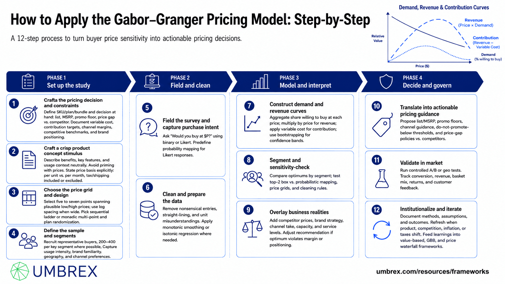
1. Clarify the pricing decision and constraints

   Define what you’re pricing (SKU, plan, bundle) and the decision at hand (list, MSRP, promo floor, price gap vs. competitor). Document constraints: variable cost, contribution targets, channel margins, competitive benchmarks, and brand positioning.

2. Craft a crisp product concept stimulus

   Describe benefits, key features, and usage context in plain language. Use visuals if relevant. Keep it neutral—avoid priming with prices. Decide and state the price basis explicitly (per unit vs. per month, tax/shipping included or excluded).

3. Choose the price grid and design

   Select a range that comfortably spans below and above plausible prices (e.g., five to seven points). Consider log spacing (e.g., 19, 29, 39, 49, 59) if the price range is wide. Pick a design variant (sequential ladder or monadic multi-point) and plan randomization to reduce anchoring.

4. Define the sample and segments

   Recruit respondents representative of target buyers. Aim for 200–400 per key segment to stabilize curves. Capture profiling attributes (usage intensity, brand familiarity, geography, channel preferences) to allow segmented curves.

5. Field the survey and capture purchase intent

   Ask “Would you buy at $P?” with a binary or Likert scale. If using a Likert scale, predefine how you’ll map responses to purchase probabilities (e.g., definitely=1.0; probably=0.7; might=0.3; probably not/definitely not=0).

6. Clean and prepare the data

   Remove nonsensical entries, check for straight-lining, and ensure prices were understood (currency, time unit). If responses were collected at multiple prices per respondent without a ladder, apply monotonic smoothing or isotonic regression so estimated demand does not increase with price.

7. Construct demand and revenue curves

   Aggregate the (weighted) share willing to buy at each price. Multiply by price for a revenue curve; apply variable cost to estimate contribution. Identify the revenue- and margin-maximizing price candidates. Use bootstrapping to create confidence bands when possible.

8. Segment and sensitivity-check

   Repeat for key segments and compare optimums. Conduct sensitivity around probability mappings (top-2 box vs. probabilistic), price grids, and data cleaning rules to assess robustness.

9. Overlay business realities

   Superimpose competitor prices, brand strategy, channel take, and operational considerations (capacity constraints, service levels). If the model’s optimum violates margin floors or positioning, adjust the recommendation or revisit the offer design.

10. Translate into actionable pricing guidance

    Propose list/MSRP, promotional floors, and channel guidance. Define guardrails (e.g., “Do not promote below $X”), and price-gap policies versus key competitors. Align internal stakeholders on the rationale and any exceptions policy.

11. Validate in market

    Run controlled A/B or geo tests where feasible. Track conversion, revenue, basket mix, returns, and customer feedback. Confirm real-world elasticity around the recommended price; refine as needed.

12. Institutionalize and iterate

    Document methods, assumptions, and outcomes. Refresh Gabor–Granger when the product changes materially, the competitive set shifts, or macro conditions (inflation, taxes) move. Feed learnings into broader pricing frameworks (value-based, Good–Better–Best) and the price waterfall.

6. Example: Gabor–Granger in Action

Company: “ArcWave Audio,” a $300M D2C consumer electronics brand preparing to launch a new pair of wireless earbuds. They needed an MSRP and a promotional floor that balanced premium positioning with volume goals ahead of holiday season.

Problem: Competitors clustered at $79, $99, and $129. ArcWave’s product offered active noise cancellation, long battery life, and splash resistance. Internally, variable cost per unit was $38; retail channel margins and promotions could reduce pocket price by 30–40% from MSRP if not carefully managed.

Applying the model:

• Stimulus and sample: A concept page and 30-second video were shown to 1,200 respondents in the US (balanced by age and income, screened for purchase intent in the category). Segments: brand-aware vs. unaware; heavy travelers vs. casual listeners.
• Price grid and design: Monadic multi-point across five prices: $59, $79, $99, $119, $139. 5-point intent scale mapped to probabilities: definitely=1.0; probably=0.7; might=0.3; probably not/definitely not=0. Randomized order to reduce anchoring.
• Results: Overall probabilistic demand estimates: 52% at $59; 42% at $79; 33% at $99; 24% at $119; 17% at $139. Revenue per 100 prospects peaked at $99 ($3,267) and remained near-peak at $119 ($2,856). Contribution (after $38 unit cost, before channel) peaked at $119. Brand-aware and traveler segments showed higher willingness to pay, with a revenue peak at $119.
• Business overlay: Considering retailer margin structures and planned promos, an MSRP of $119 with a promotional floor at $89 preserved both positioning and margin. DTC channel targeted $109–$119 with value-added bundles rather than deep discounts.

Outcome: ArcWave launched at MSRP $119, with DTC at $109 and a holiday promo at $99 (value bundle versus straight price cut). Conversion and revenue outperformed the $99 list-price scenario in A/B geo tests. Retail sell-through was strong without excessive discounting; pocket margins held within targets. The team operationalized a promo guardrail of “no offers below $89” to avoid value erosion.

7. Strengths and Limitations

Strengths

• Fast and intuitive: Simple to design and interpret; useful when you need a read quickly.
• Demand and revenue curves: Produces tangible curves to identify revenue- and margin-maximizing price candidates.
• Segmentable: Easy to run by cohort (usage, brand familiarity, geography) to tailor pricing or packaging.
• Practical for guardrails: Helps set promo floors and MSRP guidance before live tests.

Limitations

• Univariate: Varies only price; does not capture attribute trade-offs, competitive reactions, or bundling effects.
• Hypothetical bias: Stated intent can diverge from real behavior; calibration or in-market validation is essential.
• Anchoring and design sensitivity: Sequential ladders can bias results; poor price grids can put optima at the boundary.
• Brand and context effects: Results depend on stimulus clarity and whether brand equity is incorporated.

8. Common Pitfalls (and How to Avoid Them)

• Narrow or mis-specified price range
  What goes wrong: The “best” price sits at the lowest or highest tested point.
  How to avoid: Include prices below and above plausible levels; use log spacing if the range is wide.
• Anchoring in sequential ladders
  What goes wrong: Starting high or low skews ceilings.
  How to avoid: Randomize starting points or use monadic multi-point designs; counterbalance order.
• Ambiguous price basis
  What goes wrong: Respondents mix “per month” and “per year,” or tax-in vs. ex-tax; curves are noisy.
  How to avoid: Specify unit, term, and whether prices include tax/shipping; localize currency.
• No probability mapping
  What goes wrong: Treating all “probably” as definite purchases overstates demand.
  How to avoid: Define and sensitivity-test probability weights; compare to top-2 box thresholds.
• Ignoring monotonicity
  What goes wrong: Estimated demand increases with price at some points, undermining credibility.
  How to avoid: Apply monotonic smoothing/isotonic regression; increase sample sizes at each price.
• Using Gabor–Granger for complex offers
  What goes wrong: Results miss key attribute trade-offs; lead to mispricing.
  How to avoid: Use conjoint/DCE for multi-attribute optimization; keep Gabor–Granger for simpler or single-SKU cases.
• Neglecting economics and channel
  What goes wrong: The “optimal” price is unprofitable after trade terms or rebates.
  How to avoid: Overlay variable costs and a price waterfall to test pocket price robustness.
• No in-market validation
  What goes wrong: Stated-intent optimum underperforms in reality.
  How to avoid: A/B or geo test recommended prices; iterate based on behavioral data.

9. How the Gabor–Granger Pricing Model Relates to Other Frameworks

• Van Westendorp Price Sensitivity Meter (PSM): PSM maps perception thresholds and acceptable ranges (PMC–PME, OPP, IPP). Gabor–Granger estimates demand and revenue at discrete prices. Use PSM to set perception guardrails and Gabor–Granger to locate demand and revenue peaks.
• Conjoint/Discrete Choice Experiments (DCE): Conjoint models attribute trade-offs and price sensitivity together—better for complex or competitive contexts. Use Gabor–Granger for quick, single-offer pricing; use conjoint for full offer and portfolio optimization.
• Value-Based Pricing (VBP) and EVC: VBP provides the strategic anchor (price as a share of economic value vs. the next-best alternative). Use Gabor–Granger to ensure your price is acceptable to the market and to calibrate near-term list and promo policies.
• Good–Better–Best (GBB): Gabor–Granger can inform tier price gaps by estimating demand at candidate tier prices for target segments; use conjoint for feature-to-tier assignment.
• Price Waterfall: Pair Gabor–Granger’s list price recommendation with a waterfall analysis to ensure channel rebates, discounts, and freight still yield target pocket margins.
• A/B and Geo Testing: The behavioral complement. Use experiments to validate Gabor–Granger recommendations in live channels before scaling.

Choosing the right tool: If you need a fast, single-product price read, use Gabor–Granger. If you need perception guardrails, add PSM. If you’re optimizing bundles, features, and competitive positioning, use conjoint/DCE and anchor to VBP/EVC.

10. Key Takeaways

• The Gabor–Granger Pricing Model estimates demand and revenue at discrete prices by asking purchase intent, enabling quick, data-backed price recommendations.
• It is best for relatively simple offers and early-stage list/MSRP and promo decisions; it is univariate and should be complemented for complex portfolios.
• Design choices matter: clear stimulus, correct price basis, a well-spanned grid, randomization, and proper probability mapping and smoothing.
• Always overlay economics and channel terms, then validate recommendations with in-market tests before scaling.
• Use alongside PSM (perception guardrails), VBP (strategic anchor), the price waterfall (realization), and A/B testing (behavioral proof).

11. FAQs About the Gabor–Granger Pricing Model

How many price points should we test?
Five to seven well-chosen price points typically balance precision and respondent fatigue. Ensure the range spans below and above plausible prices; consider log spacing for wide ranges.

What sample size do we need?
For stable curves, target 200–400 respondents per key segment. If using a single-point monadic design with multiple price cells, ensure each price cell has at least 100–150 completes for directional reliability.

How do we convert intent scales into demand?
Define a mapping up front (e.g., definitely=1.0; probably=0.7; might=0.3; probably not/definitely not=0). Sensitivity-test your mapping and compare with a top-2 box approach. Calibrate to observed conversion when in-market data becomes available.

Is Gabor–Granger suitable for B2B?
Yes—for simpler, transactional B2B offers (self-serve tools, add-ons, standard services). For complex, multi-stakeholder solutions, prefer value-based pricing, ROI cases, and conjoint/DCE. Always complement with field validation.

How long does a Gabor–Granger study take?
A focused study can be designed, fielded, and analyzed in 1–3 weeks depending on recruitment and segmentation complexity. Add time for in-market testing and stakeholder alignment before finalizing price.

How do we account for channel margins and promotions?
Overlay a price waterfall on top of Gabor–Granger outputs to translate list/MSRP into pocket price after discounts, rebates, and freight. Set promotional floors that preserve margin and avoid perceived value erosion.